How to Evaluate Camera Sensitivity
Comparing camera performance using the EMVA1288 imaging performance standard
What's inside:
- Introduction to imaging performance measurements based on EMVA1288
- Definition of the various measurements and how they are being measured
- Comparing low light performance of cameras at different exposure times
- Comparing a traditional CCD with a modern CMOS sensor
- Comparing Sony Pregius sensor generations
- Conclusion
Comparing basic camera specifications such as frame rate, resolution and interface is easy; use our new camera selector to filter and sort 14+ EMVA Specifications to find the exact match for your project requirements. However, comparing imaging performance of cameras such as quantum efficiency, temporal dark noise and saturation capacity tends to be a little more complicated. First, we need to understand what these various measurements really mean.
What is quantum efficiency and is it measured at the peak or at a specific wavelength? How is signal to noise ratio different from dynamic range? This white paper will address these questions and will explain how to compare and select cameras based on the imaging performance data following the EMVA1288 standard.
EMVA1288 is a standard that defines what aspects of camera performance to measure, how to measure them and how to present the results in a unified method. The first section of the white paper will help to understand the various aspects of imaging performance of an imaging sensor. It will outline the basic concepts that are important to understand when considering how an image sensor converts light into a digital image and ultimately defines the performance of the sensor. Figure 1 presents a single pixel and highlights these concepts.
![]()
Figure 1: How an image sensor converts light into a digital image
First we need to understand the noise inherent in the light itself. Light consists of discrete particles, Photons, generated by a light source. Because a light source generates photons at random times, there will be noise in the perceived intensity of the light. The physics of light states that the noise observed in the intensity of light is equivalent to the square root of the number of photons generated by the light source. This type of noise is called Shot Noise.
It should be noted that the number of photons observed by a pixel will depend on the exposure times and the light intensity. This article will consider the number of photons as a combination of exposure time and light intensity. Similarly, Pixel Size has a non-linear effect on the light collection ability of the sensor because it needs to be squared to determine the light sensitive area. This will be discussed in more detail in the next article in the context of comparing performance of two cameras.
The first step in digitizing the light is to convert the photons to electrons. This article does not get into how sensors do this, rather it presents the measure of the efficiency of the conversion. The ratio of electrons generated during the digitization process to photons is called Quantum Efficiency (QE). The example sensor in Figure 1 one has QE of 50% because 3 electrons are generated when 6 photons “fall” on the sensor.
Before electrons are digitized they are stored within the pixel, referred to as the Well. The number of electrons that can be stored within the well is called Saturation Capacity or Well Depth. If the well receives more electrons than the saturation capacity additional electrons will not be stored.
Once light collection is completed by the pixel, the charge in the well is measured and this measurement is called the Signal. The measurement of the signal in Figure 1 is represented by an arrow gauge. The error associated with this measurement is called Temporal Dark Noise or Read Noise.
Finally, Grey Scale is determined by converting the signal value, expressed in electrons, into a 16-bit Analog to Digital Units (ADU) pixel value. The ratio between the analog signal value to digital grey scale value is referred to as Gain and is measured in electrons per ADU. The gain parameter as defined by the EMVA1288 standard should not be confused with the gain of the “analog to digital” conversion process.
When evaluating camera performance, it is very common to refer to Signal to Noise Ratio and Dynamic Range. These two measures of camera performance consider the ratio of noise observed by the camera versus the signal. The difference is that Dynamic Range considers only the Temporal Dark Noise, while Signal to Noise Ratio includes the root mean square (RMS) summation of the Shot Noise as well.
Absolute sensitivity threshold is the number of photons needed to get a signal equivalent to the noise observed by the sensor. This is an important metric because it represents the theoretical minimum amount of light needed to observe any meaningful signal at all. Details of this measurement will be covered in more detail in the following articles.
To help compare sensors and cameras based on the EMVA1288 standard, FLIR created an industry-first comprehensive study of imaging performance of more than 70 camera models.
| Measurement | Definition | Influenced by | Unit |
| Shot noise | Square root of signal | Caused by nature of light | e- |
| Pixel size | Well, pixel size… | Sensor design | µm |
| Quantum efficiency | Percentage of photons converted to electrons at a particular wavelength | Sensor design | % |
| Temporal dark noise (Read noise) | Noise in the sensor when there is no signal | Sensor and camera design | e- |
| Saturation capacity (Well depth) | Amount of charge that a pixel can hold | Sensor and camera design | e- |
| Maximum signal to noise ratio | Highest possible ratio of a signal to all noise included in that signal, including shot noise and temporal dark noise.” | Sensor and camera design | dB, bits |
| Dynamic range | Ratio of signal to noise including only temporal dark noise | Sensor and camera design | dB, bits |
| Absolute sensitivity threshold | Number of photons needed to have signal equal to noise | Sensor and camera design | Ƴ |
| Gain | Parameter indicating how big a change in electrons is needed to observe a change in 16bit ADUs (better known as grey scale) | Sensor and camera design | e-/ADU |
Comparing low light performance of cameras
For the purpose of this white paper, we will consider applications such as license plate recognition (LPR) or optical character recognition (OCR) where monochrome imaging is commonly used and the amount of light that camera can collect may be limited due to short exposure times. It is fairly straight forward to determine the resolution, frame rate and field of view required to solve an imaging problem, however deciding whether the camera will have sufficient imaging performance can be more difficult.
This challenge is typically solved by trial and error. Let’s consider an example where a vision system designer determines that a VGA camera with ¼’’ CCD running at 30 FPS is sufficient in the application. The initial tests may show that the camera has sufficient sensitivity at exposure times of 10 ms when the object is stationary. See Figure 2 showing a simple example with characters B,8, D and 0 that can be easily confused by a vision algorithm. The top left image taken with a ¼’’ CCD camera produces images suitable for image processing.
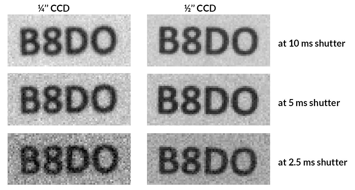
Figure 2: Results obtained from a 1/4'' and 1/2'' CCD cameras at different exposure times
However, when the object starts to move, exposure times need to be reduced and the camera is not able to provide useful information because the letter “B” and “D” cannot be distinguished from numbers “8” and “0”. Images in the middle and bottom left of Figure 2 show deterioration of image quality. In particular ¼’’ CCD at 2.5 ms exposure time produces images unsuitable for image processing.
For the purposes of this example, the assumption is that large depth of field is not required and therefore the minimum F-number of the lens is acceptable. In other words, it is not possible to collect more light by opening the shutter of the lens.
So, the designer needs to consider a different camera. The question is whether a different camera has a chance to improve the performance of the system. Using a larger sensor has generally been accepted as a good way of solving low light performance problems, so a ½’’ sensor could be a good choice. But instead of continuing with trial and error, considering the EMVA 1288 imaging performance of the camera can be useful.
| Camera | Sensor | Pixel Size (μm) | Quantum Efficiency (%) | Temporal Dark Noise (e-) | Saturation Capacity (e-) |
| 1/4’’ Camera (FL3-GE-03S1M-C) |
ICX618 | 5.6 | 70 | 11.73 | 14,508 |
| 1/2’’ Camera (BFLY-PGE-03S3M-C) |
ICX414 | 9.9 | 39 | 19.43 | 25,949 |
Looking at the EMVA 1288 data, it can be observed that ¼’’ sensor has better quantum efficiency and lower noise, but that ½’’ CCD has a larger pixel and larger saturation capacity. This article shows how to determine whether the ½’’ camera will perform better.
Figure 3 compares the cameras by plotting the signal value versus the light density (photons/ µm2). The signal as a function of light density is determined using the following formula:

An important assumption made by this article is that the lenses have the same field of view, same F-number and same camera settings.
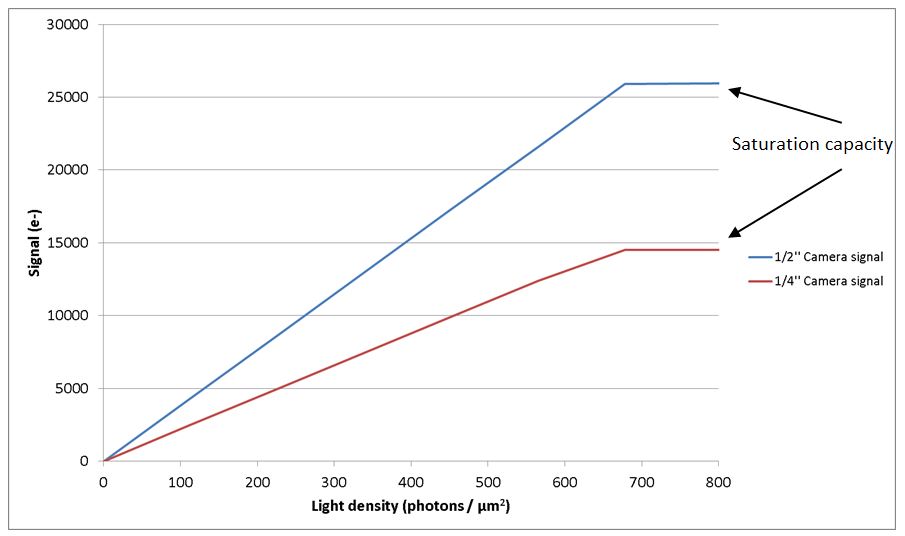
Figure 3: Signal produced by 1/4'' and 1/2'' CCD cameras as a function of the light level
Sign Up for More Articles Like This
The figure shows that for the same light density, the ½’’ sensor will generate higher signal. It can also be observed that saturation occurs at a similar light density level of 700 photons/µm2, however the ½’’ sensor has significantly higher saturation capacity.
In the application that is considered in this white paper, the comparison of cameras needs to be done at low light level. Therefore considering the noise levels becomes particularly important.
Figure 4 shows the signal and noise at low lighting levels. The noise presented in the figure is an RMS summation of Temporal Dark Noise and Shot Noise which was calculated using the following formula:
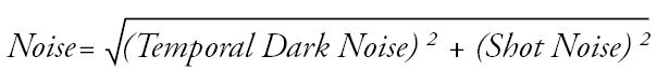
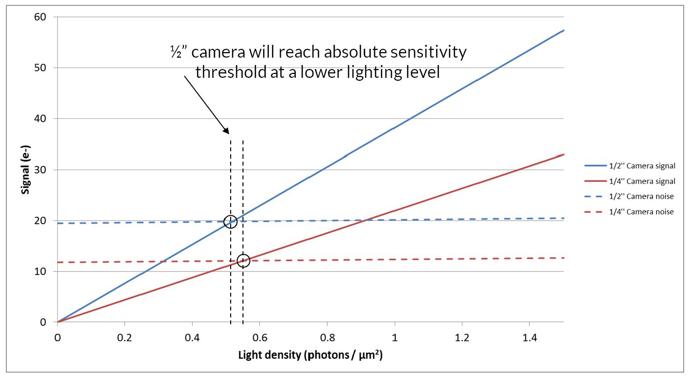
Figure 4: Signal and noise of the 1/4'' and 1/2'' CCD cameras at low light levels
The graph shows that absolute sensitivity threshold (the light level at which signal is equal to the noise) is reached by the ½’’ sensor at a slightly lower level than that of ¼’’ sensor. The more important measure needed to determine which camera will perform better in low light applications is the signal to noise ratio (SNR).
Figure 5 shows the SNR of the two cameras as a function of lighting level.
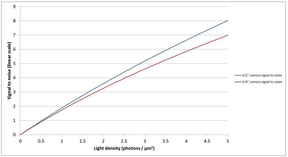
Figure 5: Signal to noise ration of the 1/4'' and 1/2'' CCD cameras at low light levels
Based on the higher signal to noise ratio of the ½’’ sensor, theory suggests that the ½’’ cameras should perform better than ¼’’ camera at low light levels.
From images in Figure 2, it can be seen that at 2.5 ms exposure time, the ½’’ sensor preserves the shape of the characters at all exposure times, while the ¼’’ sensor makes it difficult to distinguish between characters. The ½’’ sensor therefore performs better and the practical results are in-line with the theory.
FLIR has done an extensive study of cameras and has published the EMVA 1288 imaging performance results. This information can be used to compare the performance of different camera models. While camera implementation does influence the imaging performance, this study can be generally useful when comparing any two cameras with sensors that are covered in the document.
FLIR offers specific camera comparison documents. Please contact mv-info@flir.com to request a comparison between FLIR’s camera models.
It should be noted that the method outlined in this white paper is useful to get a general idea of how well a camera will perform compared to another. This method can assist in ruling out cameras that are not likely to improve the required performance, however, the ultimate test of the performance of the camera is in the actual application.
Comparing a traditional CCD with a modern CMOS sensor
Now we will compare the performance of a traditional CCD sensor versus a modern CMOS sensor in low light imaging conditions and in a scene with a wide range of lighting conditions.
In the previous section we showed that a camera with the Sony ICX414, a ½’’ VGA CCD, performs better in low light conditions than a camera with the Sony ICX618, a ¼’’ VGA CCD. Now we will compare the ½’’ VGA CCD with the new Sony Pregius IMX249, 1/1.2’’ 2.3Mpix global shutter CMOS sensor.
At first glance, this may seem like comparing “apples to oranges”, however the cost of the cameras with these two sensors is comparable at approximately €400, a VGA region of interest in the CMOS camera is actually closer to the optical size of the ¼’’ camera and the frame rates are also similar at the VGA resolution.
The EMVA 1288 data for the cameras shows that the IMX249 CMOS sensor has significantly better quantum efficiency, lower noise and higher saturation capacity. On the other hand the ICX414 CCD sensor has a larger pixel, which was the critical parameter in the example presented in the previous article.
| Camera | Sensor | Pixel Size (μm) | Quantum Efficiency (%) | Temporal Dark Noise (e-) | Saturation Capacity (e-) |
| 1/2" CCD Camera (BFLY-PGE-03S3M-C) |
ICX414 | 9.9 | 39 | 19.43 | 25,949 |
| 1/1.2" CMOS Camera (BFLY-PGE-23S6M-C) |
IMX249 | 5.86 | 80 | 7.11 | 33,105 |
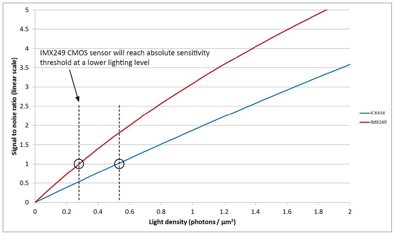
Figure 6: Signal to noise ratio of the ICX414 CCD and IMX249 CMOS sensors at low light levels
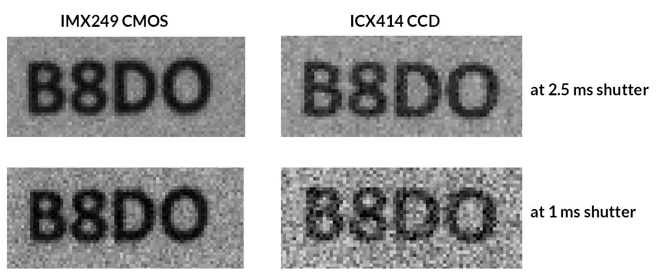
Figure 7: Results obtained from the ICX414 CCD and IMX249 CMOS sensors at different exposure times
The more interesting comparison is at higher light intensities due to the difference in the saturation capacity between the two sensors. Figure 8 shows the signal as a function of light intensity across the full range of light intensities. From the graph it can be observed that the ICX414 CCD sensor will reach saturation capacity at around 700 photons/µm2, while the IMX249 CMOS sensor will saturate at over 1200 photons/µm2.
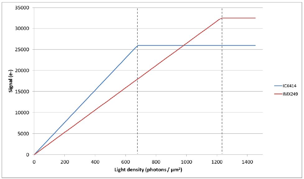
Figure 8: Signal produced by the ICX414 CCD and IMX249 CMOS sensor as a function of the light level
The first conclusion that can be made is that the image produced by the ICX414 CCD sensor will be brighter than the image produced by the IMX249 CMOS sensor. If this is not obvious from the graph, consider the image that would be produced at around 700 photons/µm2. In the case of the ICX414 CCD sensor, the image should be at the highest greyscale levels, most likely saturated, while the IMX249 CMOS sensor would produce an image that is just over 50% of the maximum brightness. This observation is significant because a naïve approach to evaluating camera sensitivity is by observing the brightness of the image. In other words, the assumption is that a brighter image will come from a camera with better performance. This however is not true and in this example it is actually the opposite, the camera that produces darker images actually has better performance.
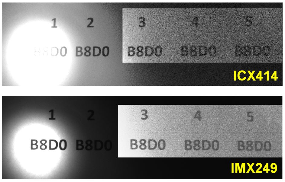
Figure 9: Results obtained with the ICX414 CCD and IMX249 CMOS sensors under difficult lighting conditions
The second observation is that the IMX249 CMOS sensor will produce images that are useful for image processing in a wider range of lighting conditions. Figure 9 shows the same scene imaged by the two cameras. It should be noted that the darker portion of the images have been enhanced for display purposes, however the underlying data was not modified. From the images it can be observed that the ICX414 CCD is saturated in the bright areas of the scene, while at the same time it has too much noise in the dark areas for the characters to be legible. On the contrary, the IMX249 CMOS sensor is producing legible characters in the bright and dark parts of the scene.
Finally, we can conclude that the recent global shutter CMOS technology has become a viable alternative to CCDs in machine vision applications. Not only are the sensors less expensive, have higher frame rates at equivalent resolutions, and do not have artifacts such as smear and blooming, but they are also exceeding the imaging performance of CCDs.
Comparing Sony Pregius generations
As we went over in the earlier section, sensor size impacts sensor performance greatly due to the fact that bigger pixels allows higher maximum number of photons to be collected in them, as well as allow more photons to be collected under the same lighting condition. The trade-off for having larger pixel size is that the sensor size will have to be bigger to accommodate a given resolution compared to using sensor with smaller pixel size, which increases the cost of the sensor. The figure below outlines how pixel size changed between different generations of Sony Pregius sensors.
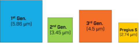
Figure 10: Pixel size differences between different generations of Sony Pregius sensors
Despite the downward trend of the pixel size (beside the 3rd generation of the sensor), the sensor’s imaging performance increased, except for sensor capacity, with each generation. A major reason for improved imaging performance is due to low temporal dark noise of the sensor found in 2nd generation onwards. The figure below outlines how the temporal dark noise of the sensor progressed through different generation of the Pregius sensor.
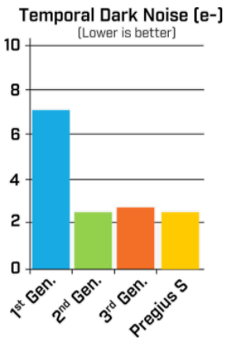
Figure 11: Pregius S maintains a low level of read noise
To get full view of the sensor imaging performance, please refer to the table below for specification of representative sensor from each Pregius generation.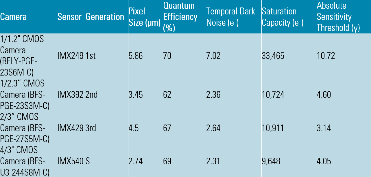
By observing the table above, one can notice that despite having the smallest pixel size, the imaging performance of the Pregius S sensor is comparable to 2nd and 3rd generation sensors, this is due to the back illuminated design of the sensor which allows for wider angle of entry for the photon that helps to capture more light onto the pixel.
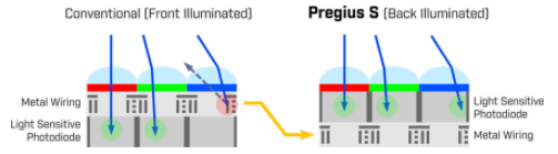
Figure 12: BSI sensors invert the traditional front illuminated sensor design making it easier for photons to enter each pixel’s light sensitive photodiode
This new sensor design allows Pregius S sensor family to maintain the imaging performance of previous generations while utilizing smallest pixel yet, leading to higher resolution sensors at relatively low prices.
Conclusion
In this white paper we learned the key concepts used in evaluating camera performance. We introduced the EMVA1288 standard and applied the results to compare camera performance under a variety of lighting conditions. There are still many more aspects of camera performance that can be considered when evaluating cameras. For example, quantum efficiency changes dramatically at different wavelengths, so a camera that performs well at 525nm, may not perform nearly as well when the light source is at near infra-red (NIR) frequencies. Similarly, long exposure times common to fluorescence and astronomic imaging need to consider the effects of dark current, a type of noise that is important at extremely low light levels.
Selecting the right camera based on imaging performance characteristics is not easy, however we hope that this white paper has helped a bit to make sense of this fascinating and complex topic.
Filter and sort using over 14 EMVA Specifications to find the exact match for your project requirements – Try our new camera selector.
See More Machine Vision
Related Articles
-
 Embedded Vision
Streaming 4x Cameras with Small Carrier Board: Fast Prototype
Read the Story -
 Embedded Vision
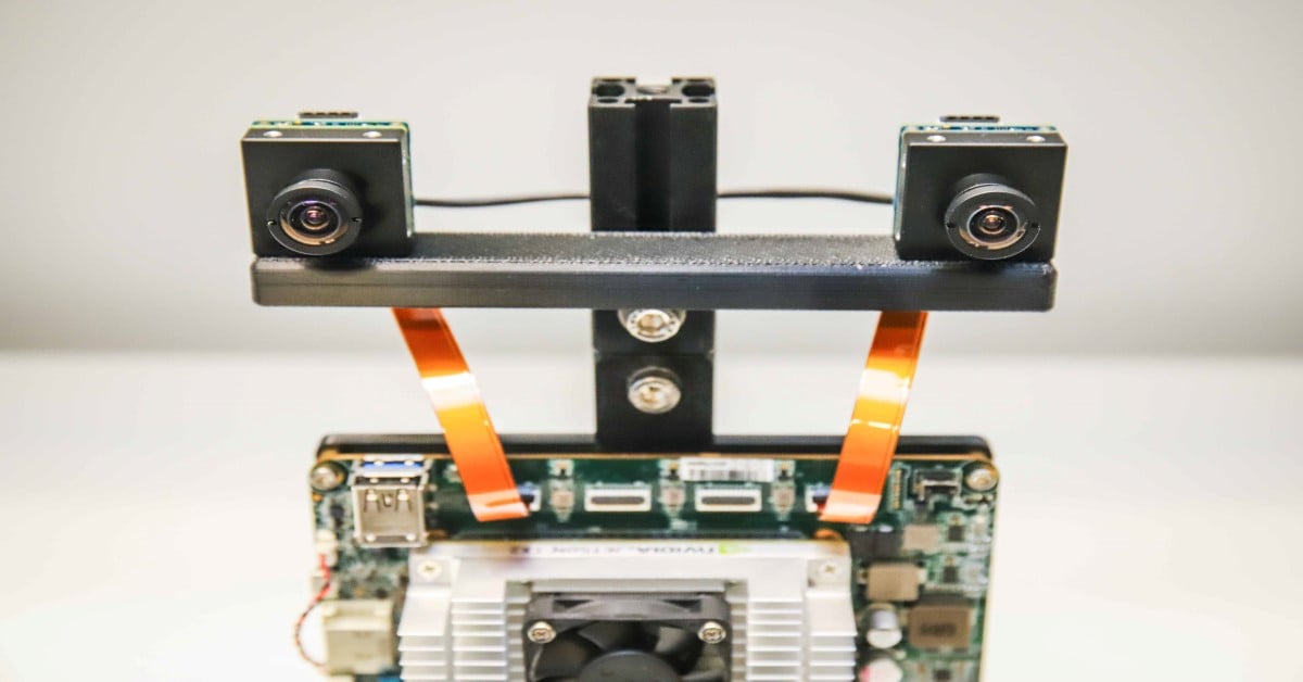
How to Build a Custom Embedded Stereo System for Depth Perception
Learn more -
 Embedded Vision
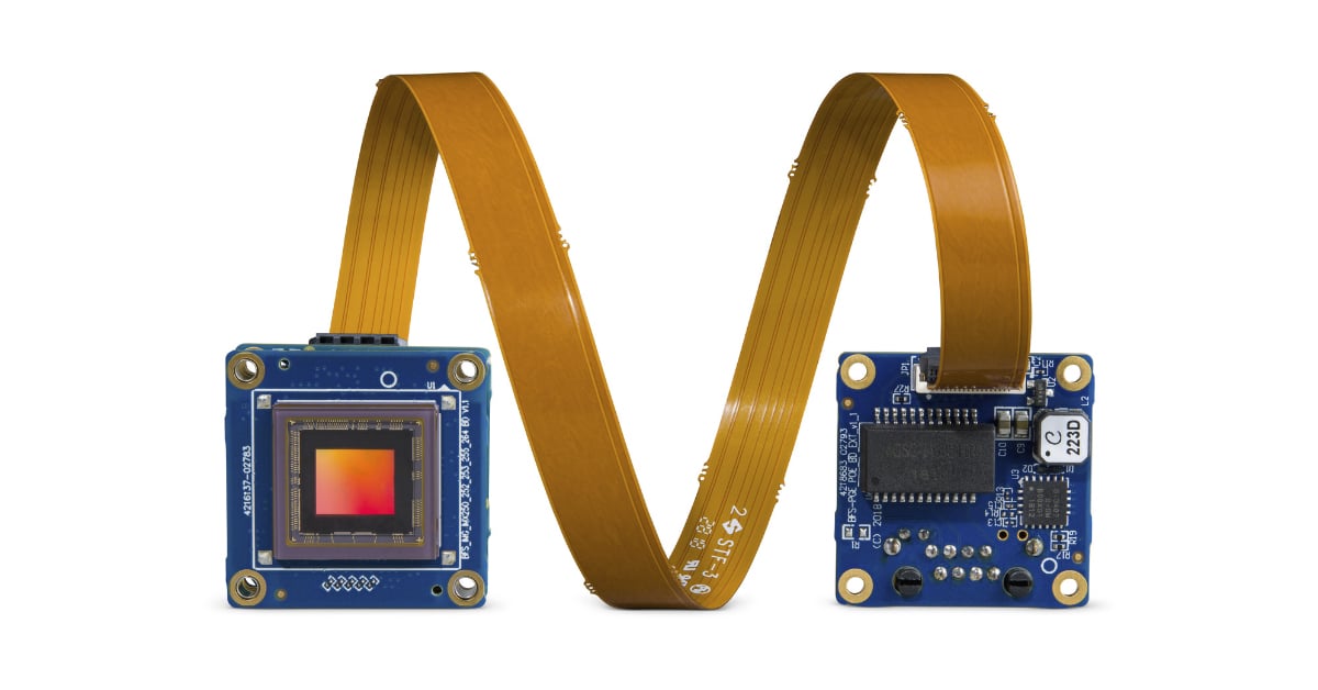
Guide for Integrating Board Level Cameras
Read the Story